VdM Plotting Inner Workings

This section will discuss everythin related to the inner workings of the plotting tools. It will go over the problem it tries to solve and how it solves it. Next, a deeper look at how all the moving parts are interconnected will be given. Finally, the section will end with a discussion on how the plotting tools should evolve in the future as well as provide the example promised in the Creating a new plugin section of the quickstart.

The Problem 

The creation of plots is a very common task in data analysis. However, every plotting script has to do a lot of work that is not directly related to the actual plotting. This includes things like:

Reading the data to memory: With the current results folder structure, parsing all the folders, reading the data and storing it in memory is a lot of work. This is especially true if the data is stored in multiple files.
Iterating over all the necessary data: Normally, one needs to iterate ovar some fits, corrections and detectors before even starting to plot. This is a lot of boilerplate code that is not directly related to the actual plotting. This, in turn, makes the code harder to read and understand and makes it more likely to contain bugs.
Code dupilication: Since the last 2 points are so common, it is very likely that the same code will be written over and over again. This is not only a waste of time, but also makes it harder to maintain the code and makes it more likely to contain bugs.

Overall, this makes the analysis of the results a lot harder than it should be

Components of the Solution 

Having understood the problem, we can now look at what a solution should look like. The solution should:

Remove boilerplate code: The solution should remove all the boilerplate code that is not directly related to the actual plotting. This includes reading the data to memory, iterating over the data and so on.
Centralize the plotting code: The solution should encourage the centralization of the plotting code. This means that the plotting code should be in one place and not spread out over multiple files.
Allow for high costumizability: The solution should allow for a high degree of costumizability. This means that the user should be able to change the plotting code to his/her liking without having to change the code of the solution itself.

This is exactly what the plotting tools do!

The Moving Parts 

The implemented solution consists of 3 main parts:

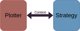
The Plotter: Soul driver of the VdM plotting framework. It takes care of all the boilerplate code that has to do with iterating over the data. This component is ignorant of the actual plotting code and data. Its job is simply to perform the necessary iterations and pass the data to the plotting strategy.
The Plotting Strategy: This component is responsible for the actual plotting. It is the only component that is aware of what the data is and how to plot it. This component indicates to the plotter how it should be used to arrive at the desired plot. This component is also responsible for providing the user with the necessary information to costumize the plot.
The Plot Context: The previous 2 components must be connected somehow. This is done by the plot context. This is a mere container that may be used to establih a communication between the plotter and the plotting strategy. It also serves the porpuse of providing the user an entry point to costumize the plot by providing the necessary via the plot context.

The Plotter 

In more detail, the plotter is responsible for:

Performing all the necessary iterations over the data: Since the plotter is unware of the actual data, it it must ask the plotting strategy for the iterators it should consider.
Allowing the plotting strategy to perform some actions at specific points in the iteration loops: Once again, the plotter only alloes for such actions to be performed. It is up to the strategy to decide whether it wants to perform any actions or not.
Updating the plot context with the current value of every iterator: This is done so that the plotting strategy can access these values and use them for the plot.

It is NOT responsible for:

Interacting with the data in any way: Any assumptions that are made by the plotter about the data will hinder the plotter’s ability to be used with different data. Eventually some assumptions could be made if the context of the plotter is well defined. However, such assumptions need to be well thought!

The Plotting Strategy 

The plotting is the component that holds must of the logic of the plot. This allows for every information about the plot to be in one place. This component is responsible for:

Specifying the iterators that the plotter should consider: This is done by implementing the iterators attribute and the get_iterators() method. The former is used to specify the iteration:
- Name: What name should be used to refer to the iterator. This will impact the name of the variable in the plot context.
- Order: What order should the iterations be performed in.
- Filters: What filters should be applied in each iteration. This is useful to avoid iterating over unnecessary data.
The latter is used to get the actual iterators. The plotter will need both these pieces of information to perform the iterations correctly.

See also

The documentation of iterations and get_iterators() for more information.
Specifying when to take an action: This is done by implementing the hook_scheme attribute.

See also

The documentation of hook_scheme for more information.
Implementing all the actions: This is done by implementing the:
- prepare() method: A default implementation is provided. However, it can be overriden if necessary.
- plot() method: Must be implemented by the user. This is where the actual plotting happens.
- style() method: A default implementation is provided. However, it is very minimal and should be overriden if necessary.
- save() method: A default implementation is provided. It is not recommended to override this method even though it is possible.
See also

The documentation of prepare(), plot(), style() and save() for more information.
Providing the user with the necessary information to costumize the plot: Am effort to force the developer to document the plot strategy has been made. However, since all the customization comes from the use of the plot context, is is possible to simply read the code of the strategy to understand where the customization points are.

The Plot Context 

The plot context is a mere container that is used to establish a communication between the plotter and the plotting strategy. It is also used to provide the user with an entry point to costumize the plot.

Important

There is only one assumption made about the plot context. It must be a dictionary-like object. In more technical terms, it must implement the MutableMapping interface.

Future Development 

Future development of these tools such take in to account the relationship between the plotter and strategy. It is imperative that the plotter and strategy are as decoupled as possible. This will allow for the plotter to be used with different strategies and for the strategies to be used with different plotters. This will also allow for the plotter to be used with different data.

Example Implementation 

Now that the inner workings of the plotting tools have been discussed, we will move on to the implementation of a plot strategy.

Note

This strategy is implemented in the plugins directory under the name of DetectorRatio.

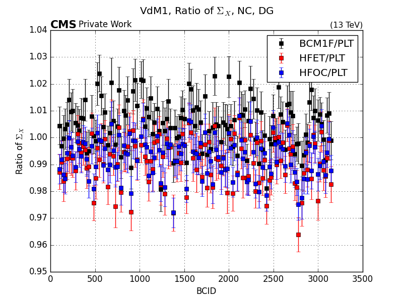
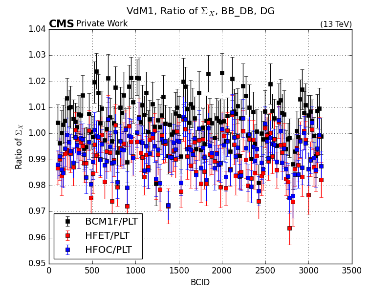
This plot strategy is used to plot the ratio of a quantity between two detectors. Like any other strategy, we start by executing the vdmplugin like

$ vdmplugin create

and go through the steps of creating a new plugin. For reference here are the answers to the questions asked by the vdmplugin script:

What should we call your plugin?.
Plugin name: MyDetectorRatio
Give a short description of your plugin.
Plugin description: Plots the ratio of a quantity given a reference detector.
What should we call your plugin's main module?
Module name [default: main]:
Where should we put your plugin?
Plugins path [default: ./plugins]:

This command will create a MyDetectorRatio directory in the plugins directory. Inside this directory, we will find a main.py file and a plugin.json file.

Note

The __init__.py files are only there to make the plugins directory a python package. They are not important for this guide.

The main.py should contain a template for the plugin along with some (hopefully), usefull comments.

Note

If the comments are not clear enough, please open an issue in the vdmtools repository or feel free to contribute to the via a merge request.

Steps 

The first step in the creation of the strategy is to change the name of the class. The template goves it the name GiveMeAName which is not very descriptive. We will change it to MyDetectorRatio. We can also add some global matplotlib settings at the top of the file.

# Add some global matplotlib settings here.
plt.style.use("classic")
plt.rcParams["legend.numpoints"] = 1

Second, we need to know what attributes our strategy will require. In this case, we need to know what will be our reference detector, the quantity we want to compare, the associated error and the latex representation of the quantity. Therefore, we will add the following attributes to the class __init__ method:

def __init__(
        self,
        quantity: str,
        reference_detector: str = "PLT",
        error: Optional[str] = None,
        latex: Optional[str] = None,
        work_status: Optional[str] = "",
        **kwargs
    ):
    super().__init__(self, **kwargs)

    self.error = error
    self.quantity = quantity
    self.latex = latex or quantity # If latex is not provided, use the quantity
    self.reference_detector = reference_detector
    self.work_status = work_status

Do not forget to add the following import statement to the top of the file:

from typing import Optional

Right after we defining our attributes, define the args_description attribute. In here, we will describe the arguments that the user can use to costumize the plot. The implementation of this attribute is as follows:

# Define the args_description here.
args_description = {
    "quantity": "The name of the column to plot.",
    "error": "The name of the column to use as error.",
    "latex": "The latex representation of the quantity.",
    "reference_detector": "The detector to use as reference.",
    "work_status": "The work status label to use"
}

Next, we will give values to the iterations, hook_scheme and unique_folder_name. These should be the first attributes to be filled in since they are the most important ones. For this plot, I will want my plotter to iterate over all the fits, corrections and detectors therefore, I will set the iterations attribute to:

iterations = [
    ('fits', []),
    ('corrections', []),
    ('detectors', []),
]

We also have to be aware that we want to skip a detector if it is the same as the reference detector. Therefore, we will add the following filter to the iterations attribute:

iterations = [
    ('fits', []),
    ('corrections', []),
    ('detectors', [lambda s, d, ctx: s.reference_detector == d]),
]

See also

The documentation of iterations for more information to understand what values a filter function should accept and what it should return.

The hook_scheme attribute is used to specify when the strategy methods should be called. For this plot, I will want to call the prepare every iteration of the corrections loop, the plot method every iteration of the detectors loop and the style and save once I leave the detectors loop. Therefore, I will set the hook_scheme attribute to:

hook_scheme = {
    CALL_ON_ENTRY: {
        "corrections": ["prepare"],
        "detectors": ["plot"],
    },
    CALL_ON_EXIT: {
        "detectors": ["style", "save"],
    },
}

Finally, the unique_folder_name attribute indicates where the results of the plot should be stored. For the sake of simplicity, I will set it to the name of the strategy:

unique_folder_name = "MyDetectorRatio"

Once these attributes are set, we can move on to the implementation of the methods. We will start with the get_iterators method. The implementation of this method requires knowledge of the data object. In this case, we will assume that the data object is a ScanResults object. Therefore, we will implement the method as follows:

def get_iterators(self, data: ScanResults) -> Dict[str, Iterator[str]]:
    return {
      "fits": data.fits,
      "detectors": data.detectors,
      "corrections": data.corrections,
    }

Note

Do not forget to add the following import statement to the top of the file:

from vdmtools.io import ScanResults

Note

The keys of the dictionary returned by this method must match the names of the iterations specified in the iterations attribute.

Now that we decided on using the ScanResults object, we must define the data_description attribute. This attribute is used to describe the data that the strategy will use. The implementation of this attribute is as follows:

data_description = "The data for this plugin must be a ScanResults object."

Now we have the hook methods to implement. For this strategy, we only have to implement the plot() and style() methods since there is no additional preparation to be done. The implementation of the plot() method is as follows:

def plot(self, i, data: ScanResults, context: dict):
    # Filter the data to get the current detector
    res = data.filter_results_by(
        context["current_fit"],
        context["current_detector"],
        context["current_correction"],
        context.get("fit_status", "good"),
        context.get("cov_status", "good")
    ).set_index("BCID")
    # Filter the data to get the reference detector
    ref = data.filter_results_by(
        context["current_fit"],
        self.reference_detector,
        context["current_correction"],
        context.get("fit_status", "good"),
        context.get("cov_status", "good")
    ).set_index("BCID")
    # Make the BCIDs match between the two dataframes
    # This is necessary since they may differ
    ref, res = DataframeUtils.match_bcids(ref, res)

    # If the error is not provided, assume it is zero
    if self.error is None:
      res_err = ref_err = np.zeros_like(res[self.quantity])
    else:
      res_err = res[self.error]
      ref_err = ref[self.error]

    # Calculate the ratio and propagate the errors
    yaxis = res[self.quantity] / ref[self.quantity]
    yerr = np.abs(yaxis) * np.sqrt(
        (res_err / res[self.quantity]) ** 2
        + (ref_err / ref[self.quantity]) ** 2
    )

    # Plot the data however you want
    plt.errorbar(
        res.index,
        yaxis,
        yerr=yerr,
        fmt=context.get("fmt", "o"),
        label=f"{context['current_detector']}/{self.reference_detector}",
        color=context.get("colors", ["k", "r", "b", "g", "m", "c", "y"])[i],
    )

There are several things to note here:

First, since I am making this strategy, I get to decide what data should be used with it. In this case I choose to use the ScanResults object. This way I get access to all the objects methods and attributes. I also use some numpy functions so I need to add the following import statement to the top of the file:
```
import numpy as np
```
Throughout the function, you can see that I am accessing my context with keys like current_detector. This is because the plotter will update the context with the current value of every iterator and the kwy will be prefixed with current_.
Sometimes, the context object is accessed with a get method. In this case the get method is the get method of the python dictionary. This allows me to request a value from a given key and provide a default value in case the key does not exist. This is were the user can costumize the plot. For example, the user can set the fmt key to o when calling the plotter run() method to plot the data with points. Since these kwys, polute the context object, it is mandatory to define the reserved_context_keys attribute. This attribute is used to specify which keys are reserved for the strategy and should not be used by the user. In this case, I will set it to:
```
# Define the reserved context keys here.
reserved_context_keys = {
    "fit_status": "The status of the fit to consider. See the ScanResults class for more info",
    "cov_status": "The status of the covariance matrix to consider. See the ScanResults class for more info",
    "fmt": "The format of the plot. For example, 'o' for circles.",
    "colors": "The colors (plt compatible) of the data points.",
}
```
I am using some utility functions from the DataframeUtils class. For this I need to add the following import statement to the top of the file:
```
from vdmtools.utils import DataframeUtils
```

The implementation of the style() method is as follows:

def style(self, i, data: ScanResults, context):
    plt.grid(True)
    plt.ticklabel_format(useOffset=False, axis="y")
    style.exp_label(data=True, label=self.work_status) # Feel free to add more arguments to the exp_label function

    # Create the title of the plot
    title = TitleBuilder() \
            .set_scan_name(data.scan_name) \
            .set_fit(context["current_fit"]) \
            .set_correction(context["current_correction"]) \
            .set_info(f"Ratio of {self.latex}") \
            .build()

    # Style the plot however you want
    plt.title(title)
    plt.xlabel("BCID")
    plt.ylabel(f"Ratio of {self.latex}")
    plt.legend(loc="best")

Some things to note are:

The use of the TitleBuilder class to create the title of the plot. For this I need to add the following import statement to the top of the file:
```
from vdmtools.utils import TitleBuilder
```
The use of the style module to style the plot. This module contains a subset of the mplhep package that is used to style the plots. For this I need to add the following import statement to the top of the file:
```
from vdmtools.utils import style
```

The strategy implementation is now complete. The full code can be found in the plugins directory under the name of MyDetectorRatio.

All that is needed is to create a configuration file and request to run use our strategy. This creation of a configuration file was discussed in the Learning about the existing plotting plugins section of the quickstart so we will not go over it again. Here is the configuration file I used:

from pathlib import Path #  All Paths should be Path objects not strings
from vdmtools.io import read_one_or_many #  Utility to read one or many files into ScanResults

#  A required variable in all configuration files
#  Holds the names of the plugins to load. In this case, only the 'NormalAllDetectors' plugin
plugins = ["MyDetectorRatio"]

#  A required variable in all configuration files
#  A list of dictionaries. Each dictionary represents a type of plot to be generated
plots = [
    {
        "strategy_name": "MyDetectorRatio",
        "strategy_args": {
            "quantity": "CapSigma_X",
            "error": "CapSigmaErr_X",
            "latex": r"$\Sigma_X$", #  The latex representation of the quantity
            "output_folder": Path("MyPlots"), #  Where to save the plots
            "file_suffix": "_CapSigma_X", #  The suffix to add to the file name
            "work_status": "Private Work", #  The work status to add to the plot
        },
        "context": {"fmt": "s"}, #  Give the context a format string to change the marker style
        "data": read_one_or_many( #  Let's read the data in the specified folder.
            Path("../data/8999_no_corr/analysed_data/8999_28Jun23_230143_28Jun23_232943"),
            "VdM1", # The name of the scan
            fits={"DG"} #  The fits to read. In this case, only the DG fit
        )
    },
]

Running the following command:

$ vdmplot run-config config.py -p plugins/

will produce the following plots: